London Bike Share Optimization

This project covers a variety of topics including:

• Data Cleaning & Preparation in Python
• Stochastic Simulation
• Queueing Theory Concepts
• Optimization

Data Acquisition & Initial Questions

The data for this project come in two .csv files which can be acquired from Kaggle here. If you would like to follow along with the notebook code from start to finish, you can access it as a github gist here. If you prefer to watch me go through this project from start to finish, you can watch a short series of videos on YouTube in which I do so. I’ll link to those below.

Here’s a quick look at the data we have to work with:

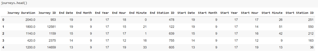
As can be seen above, we have station information as well as journey information. There are over 1.5 million journeys recorded including start time/location and end time/location.

There are two essential questions to pursue with this dataset:

1. How many bad experiences customers are having within this system?
2. How can we leverage this information for the purpose of optimizing the system and minimizing those bad experiences?

If you’ve ever been a regular user of a bike share system, you know that the two kinds of bad experience involve attempting to rent a bike at an empty dock or attempting to return a bike at a full dock.

System operators manage these issues by manually rebalancing the number of bikes at each station on a regular basis. There is a cost to all of this of course, and understanding the tradeoff between negative customer experiences and the cost of rebalancing is critical.

But there is a big piece of the puzzle missing when it comes to understanding the impact of negative experiences suffered by customers. Although we have access to rider data so that we can see when and where bikes are rented and returned, we do not have any data on the number of bad experiences suffered by customers. In order to estimate how often these bad experiences occur, we need to employ stochastic simulation methods.

Reframing the Problem

At a high level, we want to simulate a series of interactions between two random variables (customers arriving and customers departing) and two constraints (bike inventory level and the maximum capacity at each dock). If we accurately model the interactions of these random variables and simulate over the space of many thousands of instances, we should be able to determine the expected number of bad experiences occurring within the system, given certain bike inventory levels and dock capacity.

We also need to choose what interval of time is most appropriate. Using a full day as our interval of interest would cause us to lose sight of the ebbs and flows of commuter business, but using an interval of 15 minutes would likely be too granular to be very useful. For this project I’ve chosen to use one hour intervals because this gives us plenty of traffic to observe without being so broad that we lose sight of commuter trends.

Lastly, we need to accurately model the role that random order plays in the calculation of good and bad experiences. As an example of why order matters, take this simplified hypothetical:

If we somehow know there will be exactly 10 customers who drop off bikes and exactly 10 customers who pick bikes up during a certain span of time at a given dock, this gives us an unwieldy 20!/(10!*10!) = 184,756 possible order combinations. If we now assume the dock has a capacity of 10 and a beginning inventory of 5, we can see that the possible number of bad experiences may be as low as zero or as high as 5.

Without diving too far down the rabbit hole with this hypothetical, we can simply make note of the fact that calculating out the probability of X numbers of bad experiences in an empirical manner based on arrivals and departures in every combination is a complex task. It’s easiest to model our problem using Stochastic Simulation.

Data Preprocessing

In order to simulate arrivals and departures as random variables, we need to employ some queueing theory. Specifically, we need to model arrivals and departures using the Poisson distribution and we need to determine the value of Lambda in each time period of interest.

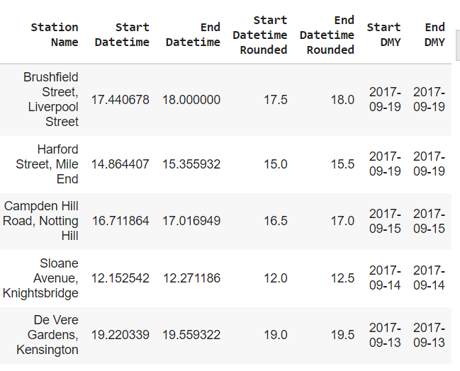
With the dataset we currently have to work with, this is a relatively simple task. First, we need to combine the time of day information into a new, single column with hour and minute together. After doing this, we can split the day up into segments of time. I’ve chosen to do this by the hour, which is admittedly a somewhat arbitrary choice. Next, we need to combine month, day and year information into a single column. Below is the code to accomplish all of this:

Our new columns end up looking like this:

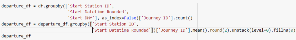
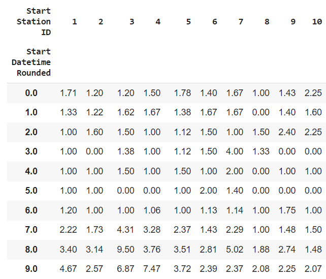
Now that we have all our necessary information in single columns, we can use a pandas groupby to organize all trips together based on where they started and when, as well as where they ended and when. Because we know the date, time, and location, we can then determine the mean average number of arrivals and departures at each station for each period of time across all days. The result here is two separate dataframes. One for mean average arrivals per station per time period, and one for mean average departures per station per time period.

Methods & Modeling

Now that we have mean averages for arrivals and departures for every hour of the day at every station in our dataset, we can use these numbers to create our Poisson distributions. Here the numbers we’ve calculated represent Lambda. In such a distribution, the probability of X arrivals during any given time period is defined as:

In this distribution, X must be a positive integer even if Lambda is a decimal of. It is also worth noting the shape of this distribution. Because the Poisson distribution has a long tail to the right, there is a built-in chance of seeing abnormally high numbers of arrivals. If you’ve ever worked in the service industry, you know from experience that those random spikes in arrivals really do occur.

Now that we understand how to model the randomness of arrivals and departures, we’re ready to write our simulation function. You can follow me through the process of writing this function in the video below, or just take a look at the code block itself if you prefer.

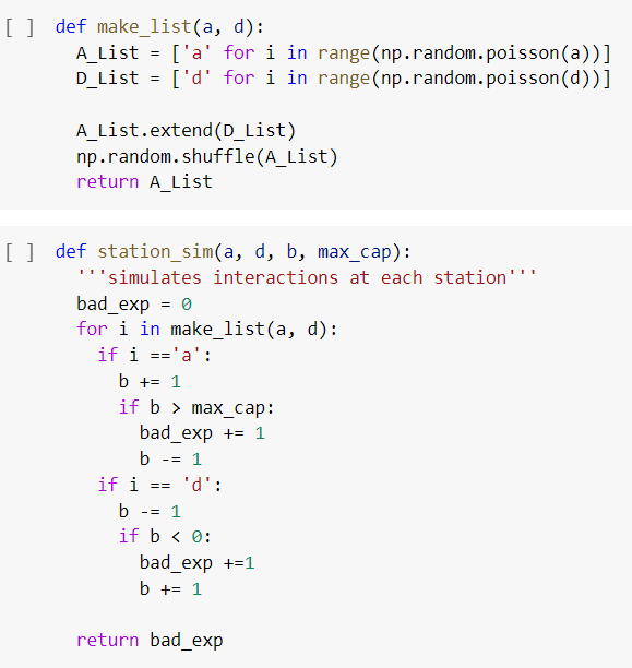
What we’re doing in the code blocks above is creating lists of characters to represent people arriving and departing in random order from a bike docking station. For each time the function is called, it samples randomly from a Poisson distribution with Lambda equal to ‘a’ for arrivals and ‘d’ for departures. It then makes lists of length equal to that random number and fills these lists with ‘a’ for arrival and ‘d’ for departure. After shuffling all characters together in a random order, our function iterates through the master list and tracks bike inventory levels. If a customer arrives to drop a bike off at a full station, or attempts to rent a bike at a station which is empty, a bad experience is recorded.

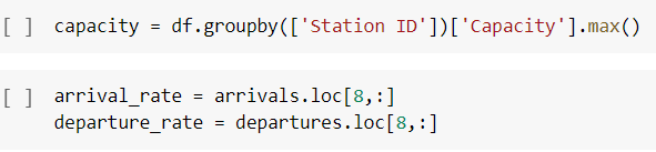
The next step is to put this function to work. The required arguments here include arrival rate, departure rate, and capacity as well as initial bike inventory levels. The code below gives us this information for every station during the 8:00am hour.

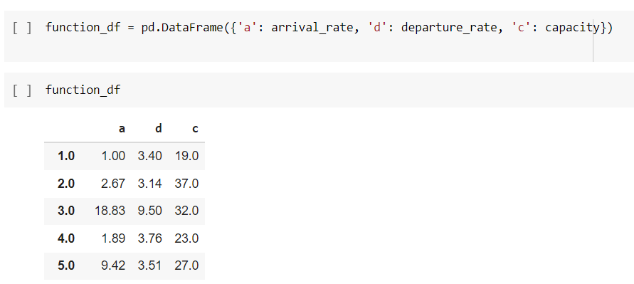
Then, we’ll create a dataframe with just the important information.

Finally, we’ll create a loop to help us simulate interactions ten thousand times at each station for each time, with every possible level of bike inventory. The output for this will provide us with the two answers we asked at the start:

1. How many bad experiences are occurring in this system based on inventory levels?
2. What are the optimal levels of inventory at each dock for each time period of the day?

Results

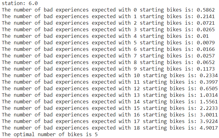
The loop above provides us with answers to the two questions we asked at the start. 1) How many bad experiences should we expect based on bike inventory levels? 2) What are optimal inventory levels per station per time period?

Here are a few snippets of the readout this loop created:

Discussion & Conclusions

As we can see from the results above, Stochastic Simulation is a good way to get answers. Intuitively, we know that optimal inventory levels are usually somewhere in the middle for these stations, but knowing exactly where they lie can be tricky. Additionally, we now have the ability to predict the number of bad experiences occurring at our stations based on inventory levels. All of this is useful.

However, there are many improvements I would make if I were to continue with this project. To begin with, what we’ve got is not easily extensible. There are well over 700 stations and 24 segments of the day to examine, which means 17,000+ possible combinations of time and place. Even just running the code above to get answers on optimal inventory levels for the 8:00am hour takes around 2 full hours while using the Google Colab GPU and high RAM options. More efficient code would help.

Additionally, my method of determining optimal levels has a flaw – it gets stuck when it reaches a solution with zero bad experiences, failing to recognize that there may be many inventory levels with zero bad experiences and the middle of those is likely the true optimal.

These issues bring me to two thoughts for future work. The first is that there must be a way of determining these expected values empirically using combinations, although admittedly I have tried and failed to discover how this would work. The second is that it may be worthwhile to employ a machine learning strategy in predicting expected values for bad experiences. In the loop I used, you may have noticed that I stored the data for each simulation in various lists. This was done with the thought that training a predictive model might be a good next step to save both time and computing power.

Thanks for following along with this! If you have questions, comments, corrections, or just want to get in touch with me. Please feel free to contact me.

gordon.e.irving@gmail.com